Normalization
In this example, the time evolution of type normalization is demonstrated. A historic emission scenario is simulated with OpenAirClim.
Imports
If the openairclim package cannot be imported, make sure that you have installed the package with pip or added the oac source folder to PYTHONPATH.
import xarray as xr
import matplotlib.pyplot as plt
import openairclim as oac

xr.set_options(display_expand_attrs=False)
<xarray.core.options.set_options at 0x7f453fb817f0>
Input files
In order to be able to execute this example simulation, three types of input are required.
Configuration file historic.toml
Emission inventory ELK_aviation_2019_res5deg_flat.nc
Time evolution file for fuel normalization time_norm_historic_SSP.nc
Emission inventory
Source: DLR Project EmissionsLandKarte (ELK)
Resolution down-sampled to 5 deg resolution
Converted into format suitable for OpenAirClim
Inventory year: 2019
inv = xr.load_dataset("source/demos/input/ELK_aviation_2019_res5deg_flat.nc")
display(inv)
<xarray.Dataset> Size: 2MB
Dimensions:   (index: 50854)
Dimensions without coordinates: index
Data variables:
    fuel      (index) float32 203kB 1.493e+04 7.459e+03 ... 7.471e+03 1.676e+03
    CO2       (index) float32 203kB 4.716e+04 2.356e+04 ... 2.36e+04 5.294e+03
    H2O       (index) float32 203kB 1.847e+04 9.227e+03 ... 9.242e+03 2.073e+03
    NOx       (index) float32 203kB 161.7 77.61 146.9 ... 965.8 134.5 23.91
    distance  (index) float32 203kB 2.266e+03 1.188e+03 ... 1.225e+03 272.1
    lat       (index) float64 407kB -67.5 -67.5 -67.5 -67.5 ... 87.5 87.5 87.5
    lon       (index) float64 407kB -167.5 -167.5 -167.5 ... 177.5 177.5 177.5
    plev      (index) float32 203kB 315.4 301.5 288.1 ... 197.5 179.4 171.0
Attributes: (9)- index: 50854
- fuel(index)float321.493e+04 7.459e+03 ... 1.676e+03
- long_name :
- fuel
- units :
- kg
array([14929.8 , 7458.867 , 12927.252 , ..., 54618.89 , 7470.914 , 1675.8184], shape=(50854,), dtype=float32) - CO2(index)float324.716e+04 2.356e+04 ... 5.294e+03
- long_name :
- CO2
- units :
- kg
array([ 47163.24 , 23562.559, 40837.188, ..., 172541.06 , 23600.617, 5293.91 ], shape=(50854,), dtype=float32) - H2O(index)float321.847e+04 9.227e+03 ... 2.073e+03
- long_name :
- H2O
- units :
- kg
array([18468.164 , 9226.618 , 15991.011 , ..., 67563.56 , 9241.5205, 2072.9873], shape=(50854,), dtype=float32) - NOx(index)float32161.7 77.61 146.9 ... 134.5 23.91
- long_name :
- NOx
- units :
- kg
array([161.68584 , 77.605194, 146.91652 , ..., 965.7742 , 134.53651 , 23.91125 ], shape=(50854,), dtype=float32) - distance(index)float322.266e+03 1.188e+03 ... 272.1
- long_name :
- distance flown
- units :
- km
array([2266.1682 , 1188.3013 , 2030.0345 , ..., 9227.67 , 1224.9799 , 272.10165], shape=(50854,), dtype=float32) - lat(index)float64-67.5 -67.5 -67.5 ... 87.5 87.5
- standard_name :
- latitude
- long_name :
- latitude
- units :
- degrees_north
- axis :
- Y
array([-67.5, -67.5, -67.5, ..., 87.5, 87.5, 87.5], shape=(50854,))
- lon(index)float64-167.5 -167.5 ... 177.5 177.5
- standard_name :
- longitude
- long_name :
- longitude
- units :
- degrees_east
- axis :
- X
array([-167.5, -167.5, -167.5, ..., 177.5, 177.5, 177.5], shape=(50854,)) - plev(index)float32315.4 301.5 288.1 ... 179.4 171.0
- standard_name :
- air_pressure
- long_name :
- pressure
- units :
- hPa
- positive :
- down
- axis :
- Z
array([315.4225 , 301.48642, 288.05444, ..., 197.46225, 179.43054,
       171.04308], shape=(50854,), dtype=float32)
- Title :
- ELK - Aviation - All subsectors Global, 2019, annual. Original data modified as stated under "Changes". Original datasets were retrieved from: https://elkis.dlr.de
- Changes :
- lon/lat regridded to 5 deg resolution, dataset flattened, emission densitities converted to absolute yearly emissions, altitude converted to units of hPa. Changes made by Stefan Völk, DLR Institute of Atmospheric Physics, https://www.dlr.de/en/pa/
- Inventory_Year :
- 2019
- comment :
- The emission inventory in final version 2.1 was developed by DLR in 2024. The methodology is based on a bottom-up approach of a global weekly flight plan for summer and winter season. Modeled aircraft trajectories followed the total energy model and used BADA aircraft performance data, emissions were derived with fuel flow correlation methods and emission factors from ICAO Aircraft Engine Emissions Databank.
- references :
- https://www.dlr.de/pa/en/desktopdefault.aspx/tabid-2342/6725_read-77021/
- version :
- 2.1
- institution :
- DLR Institute of Air Transport, www.dlr.de/lv/en/
- license :
- https://creativecommons.org/licenses/by-nc/4.0/
- Conventions :
- CF-1.8
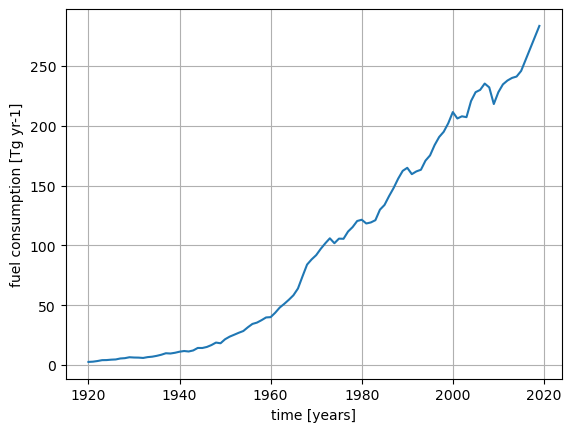
Time evolution
Time evolution with normalization of fuel use
Time period: 1920 - 2019
evo = xr.load_dataset("source/demos/input/time_norm_historic_SSP.nc")
display(evo)

fig, ax = plt.subplots()
evo.fuel.plot(ax=ax)
ax.grid(True)
<xarray.Dataset> Size: 2kB
Dimensions:  (time: 100)
Coordinates:
  * time     (time) int64 800B 1920 1921 1922 1923 1924 ... 2016 2017 2018 2019
Data variables:
    fuel     (time) float64 800B 2.669 2.889 3.427 4.145 ... 264.7 274.1 283.5
Attributes: (5)- time: 100
- time(time)int641920 1921 1922 ... 2017 2018 2019
- units :
- years
array([1920, 1921, 1922, 1923, 1924, 1925, 1926, 1927, 1928, 1929, 1930, 1931,
       1932, 1933, 1934, 1935, 1936, 1937, 1938, 1939, 1940, 1941, 1942, 1943,
       1944, 1945, 1946, 1947, 1948, 1949, 1950, 1951, 1952, 1953, 1954, 1955,
       1956, 1957, 1958, 1959, 1960, 1961, 1962, 1963, 1964, 1965, 1966, 1967,
       1968, 1969, 1970, 1971, 1972, 1973, 1974, 1975, 1976, 1977, 1978, 1979,
       1980, 1981, 1982, 1983, 1984, 1985, 1986, 1987, 1988, 1989, 1990, 1991,
       1992, 1993, 1994, 1995, 1996, 1997, 1998, 1999, 2000, 2001, 2002, 2003,
       2004, 2005, 2006, 2007, 2008, 2009, 2010, 2011, 2012, 2013, 2014, 2015,
       2016, 2017, 2018, 2019])
- fuel(time)float642.669 2.889 3.427 ... 274.1 283.5
- long_name :
- fuel consumption
- units :
- Tg yr-1
array([  2.66913509,   2.88860105,   3.42713112,   4.14475577,
         4.2179283 ,   4.55199625,   4.74136026,   5.54832768,
         5.8189377 ,   6.57585454,   6.34365569,   6.26501758,
         5.98929946,   6.68586525,   7.04860304,   7.75790222,
         8.68397285,   9.91794577,   9.70089341,  10.31627699,
        11.20736101,  11.78355837,  11.3910928 ,  12.25941114,
        14.34666505,  14.30566825,  15.180407  ,  16.75629068,
        18.83477439,  18.26746357,  21.62190288,  23.79720232,
        25.39795749,  27.03441874,  28.49608593,  31.6347463 ,
        34.42047288,  35.53556056,  37.55298606,  39.84708199,
        40.10071859,  43.76752312,  48.12050078,  51.23263118,
        54.62917133,  58.36694813,  64.05982447,  74.19600767,
        84.03846813,  88.36608656,  91.91482043,  97.18404963,
       101.81857244, 105.99496686, 101.89307962, 105.72207783,
       105.5828682 , 111.66079153, 115.37622662, 120.45269205,
       121.49723589, 118.38147706, 119.25617925, 121.13443579,
       129.92849598, 133.86353934, 141.25665965, 148.02556506,
       155.83683671, 162.38092907, 164.9168532 , 159.62949952,
       161.92851276, 163.29861346, 170.92109636, 175.29800744,
       183.89089743, 190.67468562, 195.03718131, 202.17916177,
       211.50820129, 206.15679646, 207.96960702, 207.25892444,
       220.70184815, 228.13894501, 230.04580603, 235.34230583,
       232.13888363, 218.23513108, 228.15060192, 234.66167391,
       237.89117593, 240.05906677, 241.204685  , 245.90271973,
       255.30698609, 264.71125246, 274.11551883, 283.51978519])
- Title :
- Historic aviation emissions until 2014 + SSP 2-4.5 extension until 2019
- Convention :
- CF-XXX
- Type :
- norm
- References :
- Hoesly et al. (2018), Gidden et al. (2019)
- URL :
- https://doi.org/10.5194/gmd-11-369-2018, https://doi.org/10.5194/gmd-12-1443-2019
Simulation run
oac.run("source/demos/01_norm/historic.toml")
Results
Time series
Emission sums
Concentrations
Radiative forcings
Temperature changes
results_ds = xr.load_dataset("source/demos/01_norm/results/historic.nc")
display(results_ds)
<xarray.Dataset> Size: 17kB
Dimensions:        (ac: 2, time: 100)
Coordinates:
  * ac             (ac) <U7 56B 'DEFAULT' 'TOTAL'
  * time           (time) int64 800B 1920 1921 1922 1923 ... 2016 2017 2018 2019
Data variables:
    emis_CO2       (ac, time) float64 2kB 8.432 9.125 10.83 ... 865.9 895.6
    emis_distance  (ac, time) float64 2kB 5.849e+08 6.33e+08 ... 6.213e+10
    emis_H2O       (ac, time) float64 2kB 3.302 3.573 4.239 ... 339.1 350.7
    conc_CO2       (ac, time) float64 2kB 0.001082 0.002194 ... 2.754 2.828
    RF_CO2         (ac, time) float64 2kB 1.955e-05 3.963e-05 ... 0.04412
    RF_cont        (ac, time) float64 2kB 0.000461 0.0004989 ... 0.04735 0.04897
    RF_H2O         (ac, time) float64 2kB 4.615e-05 4.995e-05 ... 0.004902
    dT_CO2         (ac, time) float64 2kB 1.489e-06 4.343e-06 ... 0.02605
    dT_cont        (ac, time) float64 2kB 2.072e-05 4.085e-05 ... 0.01742
    dT_H2O         (ac, time) float64 2kB 4.007e-06 7.9e-06 ... 0.003293 0.00337
Attributes: (4)- ac: 2
- time: 100
- ac(ac)<U7'DEFAULT' 'TOTAL'
- long_name :
- aircraft identifier
array(['DEFAULT', 'TOTAL'], dtype='<U7')
- time(time)int641920 1921 1922 ... 2017 2018 2019
- long_name :
- time
- units :
- years
array([1920, 1921, 1922, 1923, 1924, 1925, 1926, 1927, 1928, 1929, 1930, 1931,
       1932, 1933, 1934, 1935, 1936, 1937, 1938, 1939, 1940, 1941, 1942, 1943,
       1944, 1945, 1946, 1947, 1948, 1949, 1950, 1951, 1952, 1953, 1954, 1955,
       1956, 1957, 1958, 1959, 1960, 1961, 1962, 1963, 1964, 1965, 1966, 1967,
       1968, 1969, 1970, 1971, 1972, 1973, 1974, 1975, 1976, 1977, 1978, 1979,
       1980, 1981, 1982, 1983, 1984, 1985, 1986, 1987, 1988, 1989, 1990, 1991,
       1992, 1993, 1994, 1995, 1996, 1997, 1998, 1999, 2000, 2001, 2002, 2003,
       2004, 2005, 2006, 2007, 2008, 2009, 2010, 2011, 2012, 2013, 2014, 2015,
       2016, 2017, 2018, 2019])
- emis_CO2(ac, time)float648.432 9.125 10.83 ... 865.9 895.6
- long_name :
- CO2 Emission
- units :
- Tg
array([[ 8.43179776, 9.12509072, 10.82630722, 13.09328351, 13.3244355 , 14.37975617, 14.97795709, 17.52716716, 18.38202423, 20.77312451, 20.03960836, 19.79119056, 18.92019703, 21.12064835, 22.26653703, 24.50721315, 27.43267026, 31.33079073, 30.64512232, 32.58911906, 35.40405348, 37.22426095, 35.98446219, 38.72747986, 45.32111496, 45.19160607, 47.95490578, 52.93312233, 59.49905239, 57.7069175 , 68.30359129, 75.17536222, 80.2321478 , 85.40172892, 90.01913556, 99.93416368, 108.73427397, 112.25683596, 118.62988311, 125.87693218, 126.6781702 , 138.26160573, 152.01266214, 161.8438821 , 172.57355246, 184.38118938, 202.36498576, 234.38518851, 265.47752116, 279.14846779, 290.35891809, 307.00441317, 321.64487073, 334.83810074, 321.88023894, 333.97604427, 333.53628107, 352.7364409 , 364.47350035, 380.51005466, 383.80976865, 373.9670865 , 376.73027072, 382.66368315, 410.44411932, 422.8749213 , 446.22978838, 467.61276062, 492.28856779, 512.96135559, 520.97233993, 504.26958961, 511.53217245, 515.86032056, 539.93974407, 553.76640621, 580.9113457 , 602.34133263, 616.12245654, 638.68397285, ... 35.40405348, 37.22426095, 35.98446219, 38.72747986, 45.32111496, 45.19160607, 47.95490578, 52.93312233, 59.49905239, 57.7069175 , 68.30359129, 75.17536222, 80.2321478 , 85.40172892, 90.01913556, 99.93416368, 108.73427397, 112.25683596, 118.62988311, 125.87693218, 126.6781702 , 138.26160573, 152.01266214, 161.8438821 , 172.57355246, 184.38118938, 202.36498576, 234.38518851, 265.47752116, 279.14846779, 290.35891809, 307.00441317, 321.64487073, 334.83810074, 321.88023894, 333.97604427, 333.53628107, 352.7364409 , 364.47350035, 380.51005466, 383.80976865, 373.9670865 , 376.73027072, 382.66368315, 410.44411932, 422.8749213 , 446.22978838, 467.61276062, 492.28856779, 512.96135559, 520.97233993, 504.26958961, 511.53217245, 515.86032056, 539.93974407, 553.76640621, 580.9113457 , 602.34133263, 616.12245654, 638.68397285, 668.15440871, 651.24932085, 656.9759894 , 654.73094313, 697.19713918, 720.69092818, 726.71470216, 743.44634506, 733.3267343 , 689.40477994, 720.72775237, 741.29622883, 751.49822571, 758.34659287, 761.96560088, 776.8066926 , 806.51477009, 836.22284757, 865.93092506, 895.63900255]]) - emis_distance(ac, time)float645.849e+08 6.33e+08 ... 6.213e+10
- long_name :
- distance Emission
- units :
- km
array([[5.84948375e+08, 6.33044950e+08, 7.51065312e+08, 9.08334750e+08, 9.24370712e+08, 9.97582632e+08, 1.03908228e+09, 1.21593143e+09, 1.27523637e+09, 1.44111680e+09, 1.39022978e+09, 1.37299602e+09, 1.31257163e+09, 1.46522596e+09, 1.54472095e+09, 1.70016584e+09, 1.90311679e+09, 2.17354539e+09, 2.12597776e+09, 2.26084078e+09, 2.45612432e+09, 2.58239958e+09, 2.49638965e+09, 2.68668403e+09, 3.14411153e+09, 3.13512697e+09, 3.32682840e+09, 3.67218769e+09, 4.12769317e+09, 4.00336543e+09, 4.73850013e+09, 5.21522304e+09, 5.56603299e+09, 5.92466802e+09, 6.24499645e+09, 6.93284259e+09, 7.54334232e+09, 7.78771689e+09, 8.22984129e+09, 8.73259879e+09, 8.78818396e+09, 9.59177437e+09, 1.05457415e+10, 1.12277735e+10, 1.19721348e+10, 1.27912789e+10, 1.40388886e+10, 1.62602613e+10, 1.84172639e+10, 1.93656735e+10, 2.01433884e+10, 2.12981546e+10, 2.23138232e+10, 2.32290917e+10, 2.23301517e+10, 2.31692873e+10, 2.31387791e+10, 2.44707729e+10, 2.52850208e+10, 2.63975423e+10, 2.66264570e+10, 2.59436298e+10, 2.61353232e+10, 2.65469484e+10, 2.84741911e+10, 2.93365668e+10, 3.09567897e+10, 3.24402141e+10, 3.41520760e+10, 3.55862320e+10, 3.61419868e+10, 3.49832486e+10, 3.54870837e+10, 3.57873451e+10, 3.74578334e+10, 3.84170457e+10, 4.03002014e+10, 4.17868874e+10, 4.27429405e+10, 4.43081254e+10, ... 2.45612432e+09, 2.58239958e+09, 2.49638965e+09, 2.68668403e+09, 3.14411153e+09, 3.13512697e+09, 3.32682840e+09, 3.67218769e+09, 4.12769317e+09, 4.00336543e+09, 4.73850013e+09, 5.21522304e+09, 5.56603299e+09, 5.92466802e+09, 6.24499645e+09, 6.93284259e+09, 7.54334232e+09, 7.78771689e+09, 8.22984129e+09, 8.73259879e+09, 8.78818396e+09, 9.59177437e+09, 1.05457415e+10, 1.12277735e+10, 1.19721348e+10, 1.27912789e+10, 1.40388886e+10, 1.62602613e+10, 1.84172639e+10, 1.93656735e+10, 2.01433884e+10, 2.12981546e+10, 2.23138232e+10, 2.32290917e+10, 2.23301517e+10, 2.31692873e+10, 2.31387791e+10, 2.44707729e+10, 2.52850208e+10, 2.63975423e+10, 2.66264570e+10, 2.59436298e+10, 2.61353232e+10, 2.65469484e+10, 2.84741911e+10, 2.93365668e+10, 3.09567897e+10, 3.24402141e+10, 3.41520760e+10, 3.55862320e+10, 3.61419868e+10, 3.49832486e+10, 3.54870837e+10, 3.57873451e+10, 3.74578334e+10, 3.84170457e+10, 4.03002014e+10, 4.17868874e+10, 4.27429405e+10, 4.43081254e+10, 4.63526103e+10, 4.51798351e+10, 4.55771175e+10, 4.54213695e+10, 4.83674236e+10, 4.99972840e+10, 5.04151779e+10, 5.15759206e+10, 5.08738817e+10, 4.78268357e+10, 4.99998387e+10, 5.14267582e+10, 5.21345125e+10, 5.26096118e+10, 5.28606773e+10, 5.38902646e+10, 5.59512357e+10, 5.80122069e+10, 6.00731780e+10, 6.21341491e+10]]) - emis_H2O(ac, time)float643.302 3.573 4.239 ... 339.1 350.7
- long_name :
- H2O Emission
- units :
- Tg
array([[ 3.30172011, 3.5731995 , 4.23936121, 5.12706291, 5.21757731, 5.63081937, 5.86506266, 6.86328135, 7.19802596, 8.13433208, 7.84710211, 7.74982677, 7.40876345, 8.27041533, 8.71912198, 9.59652507, 10.74207444, 12.26849895, 12.00000518, 12.76123467, 13.86350561, 14.57626174, 14.09078182, 15.16489162, 17.74682472, 17.69611167, 18.77816351, 20.72753163, 23.29861598, 22.5968525 , 26.74629393, 29.43713934, 31.41727349, 33.44157607, 35.24965838, 39.13218126, 42.57812506, 43.95748852, 46.45304387, 49.29084055, 49.60458902, 54.14042624, 59.5250596 , 63.37476492, 67.5762851 , 72.19991502, 79.24200306, 91.78046171, 103.95558533, 109.30884934, 113.69863314, 120.21666969, 125.94957441, 131.11577433, 126.0417398 , 130.77821059, 130.60600828, 138.12439946, 142.72039267, 148.99998043, 150.29208116, 146.43788748, 147.51989409, 149.84329744, 160.72154992, 165.58919856, 174.73448841, 183.10762443, 192.77016748, 200.86520975, 204.00214791, 197.46169138, 200.30557077, 202.00038534, 211.42939671, 216.84363573, 227.47304067, 235.86458668, 241.26099387, 250.09562372, ... 13.86350561, 14.57626174, 14.09078182, 15.16489162, 17.74682472, 17.69611167, 18.77816351, 20.72753163, 23.29861598, 22.5968525 , 26.74629393, 29.43713934, 31.41727349, 33.44157607, 35.24965838, 39.13218126, 42.57812506, 43.95748852, 46.45304387, 49.29084055, 49.60458902, 54.14042624, 59.5250596 , 63.37476492, 67.5762851 , 72.19991502, 79.24200306, 91.78046171, 103.95558533, 109.30884934, 113.69863314, 120.21666969, 125.94957441, 131.11577433, 126.0417398 , 130.77821059, 130.60600828, 138.12439946, 142.72039267, 148.99998043, 150.29208116, 146.43788748, 147.51989409, 149.84329744, 160.72154992, 165.58919856, 174.73448841, 183.10762443, 192.77016748, 200.86520975, 204.00214791, 197.46169138, 200.30557077, 202.00038534, 211.42939671, 216.84363573, 227.47304067, 235.86458668, 241.26099387, 250.09562372, 261.63564563, 255.01595785, 257.25840451, 256.37929015, 273.00818683, 282.20787566, 284.56666275, 291.11843302, 287.15579974, 269.9568578 , 282.22229526, 290.27649134, 294.27138534, 296.95306631, 298.37019607, 304.18166504, 315.81474257, 327.44782009, 339.08089761, 350.71397514]]) - conc_CO2(ac, time)float640.001082 0.002194 ... 2.754 2.828
- long_name :
- CO2 Concentration
- units :
- ppmv
array([[1.08195296e-03, 2.19420296e-03, 3.48056133e-03, 5.01435310e-03, 6.52971190e-03, 8.14246839e-03, 9.79400342e-03, 1.17373718e-02, 1.37429720e-02, 1.60112718e-02, 1.81322346e-02, 2.01833102e-02, 2.20907585e-02, 2.42570909e-02, 2.65313934e-02, 2.90514224e-02, 3.18954149e-02, 3.51766995e-02, 3.82920787e-02, 4.15999549e-02, 4.52066313e-02, 4.89744081e-02, 5.25103273e-02, 5.63457979e-02, 6.09602158e-02, 6.54543503e-02, 7.02212782e-02, 7.55382032e-02, 8.15881498e-02, 8.72729394e-02, 9.42218640e-02, 1.01895315e-01, 1.10044584e-01, 1.18683768e-01, 1.27738407e-01, 1.37887505e-01, 1.48948627e-01, 1.60224177e-01, 1.72100163e-01, 1.84679415e-01, 1.97120548e-01, 2.10840419e-01, 2.26062341e-01, 2.42230725e-01, 2.59450356e-01, 2.77842373e-01, 2.98176592e-01, 3.22192238e-01, 3.49627130e-01, 3.78150780e-01, 4.07495487e-01, 4.38396789e-01, 4.70577251e-01, 5.03846128e-01, 5.34849101e-01, 5.66979115e-01, 5.98568811e-01, 6.32188639e-01, 6.66778177e-01, 7.02873852e-01, 7.38799121e-01, 7.72925639e-01, 8.06997994e-01, 8.41419572e-01, 8.78972827e-01, 9.17524837e-01, 9.58476178e-01, 1.00149284e+00, 1.04695312e+00, 1.09428495e+00, 1.14184577e+00, 1.18653304e+00, 1.23163301e+00, 1.27674036e+00, 1.32439462e+00, 1.37314850e+00, 1.42469608e+00, 1.47819867e+00, 1.53264106e+00, 1.58917453e+00, ... 4.52066313e-02, 4.89744081e-02, 5.25103273e-02, 5.63457979e-02, 6.09602158e-02, 6.54543503e-02, 7.02212782e-02, 7.55382032e-02, 8.15881498e-02, 8.72729394e-02, 9.42218640e-02, 1.01895315e-01, 1.10044584e-01, 1.18683768e-01, 1.27738407e-01, 1.37887505e-01, 1.48948627e-01, 1.60224177e-01, 1.72100163e-01, 1.84679415e-01, 1.97120548e-01, 2.10840419e-01, 2.26062341e-01, 2.42230725e-01, 2.59450356e-01, 2.77842373e-01, 2.98176592e-01, 3.22192238e-01, 3.49627130e-01, 3.78150780e-01, 4.07495487e-01, 4.38396789e-01, 4.70577251e-01, 5.03846128e-01, 5.34849101e-01, 5.66979115e-01, 5.98568811e-01, 6.32188639e-01, 6.66778177e-01, 7.02873852e-01, 7.38799121e-01, 7.72925639e-01, 8.06997994e-01, 8.41419572e-01, 8.78972827e-01, 9.17524837e-01, 9.58476178e-01, 1.00149284e+00, 1.04695312e+00, 1.09428495e+00, 1.14184577e+00, 1.18653304e+00, 1.23163301e+00, 1.27674036e+00, 1.32439462e+00, 1.37314850e+00, 1.42469608e+00, 1.47819867e+00, 1.53264106e+00, 1.58917453e+00, 1.64863481e+00, 1.70498443e+00, 1.76138638e+00, 1.81682638e+00, 1.87710510e+00, 1.93952155e+00, 2.00179105e+00, 2.06537456e+00, 2.12680405e+00, 2.18191126e+00, 2.24069723e+00, 2.30149363e+00, 2.36286581e+00, 2.42438785e+00, 2.48567007e+00, 2.54819027e+00, 2.61380324e+00, 2.68237104e+00, 2.75380019e+00, 2.82802248e+00]]) - RF_CO2(ac, time)float641.955e-05 3.963e-05 ... 0.04412
- long_name :
- CO2 Radiative Forcing
- units :
- W/m²
array([[1.95498316e-05, 3.96296910e-05, 6.28350970e-05, 9.04847917e-05, 1.17777929e-04, 1.46803382e-04, 1.76502357e-04, 2.11432281e-04, 2.47452020e-04, 2.88168405e-04, 3.26198830e-04, 3.62938480e-04, 3.97065180e-04, 4.35812814e-04, 4.76466074e-04, 5.21494529e-04, 5.72295913e-04, 6.30894881e-04, 6.86468067e-04, 7.45442493e-04, 8.09716470e-04, 8.76818096e-04, 9.39711567e-04, 1.00790063e-03, 1.08996436e-03, 1.16980670e-03, 1.25445276e-03, 1.34884802e-03, 1.45624435e-03, 1.55703363e-03, 1.68027277e-03, 1.81404696e-03, 1.95582889e-03, 2.10582447e-03, 2.26268378e-03, 2.43837061e-03, 2.62957189e-03, 2.82392162e-03, 3.02819867e-03, 3.24415998e-03, 3.45698901e-03, 3.69150562e-03, 3.95150491e-03, 4.22716759e-03, 4.52024730e-03, 4.83276347e-03, 5.17797942e-03, 5.58587849e-03, 6.05161427e-03, 6.53464954e-03, 7.03028469e-03, 7.55112107e-03, 8.09226791e-03, 8.65035424e-03, 9.16784507e-03, 9.70296330e-03, 1.02271592e-02, 1.07842998e-02, 1.13561808e-02, 1.19518449e-02, 1.25427432e-02, 1.31013293e-02, 1.36572548e-02, 1.42173425e-02, 1.48284597e-02, 1.54544779e-02, 1.61188495e-02, 1.68157897e-02, 1.75514737e-02, 1.83160328e-02, 1.90821779e-02, 1.97982139e-02, 2.05189615e-02, 2.12376989e-02, 2.19963549e-02, 2.27710249e-02, 2.35892826e-02, 2.44373829e-02, 2.52984824e-02, 2.61913449e-02, ... 8.09716470e-04, 8.76818096e-04, 9.39711567e-04, 1.00790063e-03, 1.08996436e-03, 1.16980670e-03, 1.25445276e-03, 1.34884802e-03, 1.45624435e-03, 1.55703363e-03, 1.68027277e-03, 1.81404696e-03, 1.95582889e-03, 2.10582447e-03, 2.26268378e-03, 2.43837061e-03, 2.62957189e-03, 2.82392162e-03, 3.02819867e-03, 3.24415998e-03, 3.45698901e-03, 3.69150562e-03, 3.95150491e-03, 4.22716759e-03, 4.52024730e-03, 4.83276347e-03, 5.17797942e-03, 5.58587849e-03, 6.05161427e-03, 6.53464954e-03, 7.03028469e-03, 7.55112107e-03, 8.09226791e-03, 8.65035424e-03, 9.16784507e-03, 9.70296330e-03, 1.02271592e-02, 1.07842998e-02, 1.13561808e-02, 1.19518449e-02, 1.25427432e-02, 1.31013293e-02, 1.36572548e-02, 1.42173425e-02, 1.48284597e-02, 1.54544779e-02, 1.61188495e-02, 1.68157897e-02, 1.75514737e-02, 1.83160328e-02, 1.90821779e-02, 1.97982139e-02, 2.05189615e-02, 2.12376989e-02, 2.19963549e-02, 2.27710249e-02, 2.35892826e-02, 2.44373829e-02, 2.52984824e-02, 2.61913449e-02, 2.71294512e-02, 2.79840914e-02, 2.88354097e-02, 2.96668416e-02, 3.05728223e-02, 3.15089164e-02, 3.24380368e-02, 3.33838816e-02, 3.42903659e-02, 3.50912417e-02, 3.59470675e-02, 3.68184523e-02, 3.76944816e-02, 3.85682027e-02, 3.94334151e-02, 4.03135304e-02, 4.12056292e-02, 4.21383226e-02, 4.31095569e-02, 4.41179198e-02]]) - RF_cont(ac, time)float640.000461 0.0004989 ... 0.04897
- long_name :
- cont Radiative Forcing
- units :
- W/m²
array([[0.00046103, 0.00049893, 0.00059195, 0.0007159 , 0.00072854, 0.00078624, 0.00081895, 0.00095834, 0.00100508, 0.00113582, 0.00109571, 0.00108213, 0.0010345 , 0.00115482, 0.00121747, 0.00133998, 0.00149994, 0.00171308, 0.00167559, 0.00178188, 0.00193579, 0.00203532, 0.00196753, 0.00211751, 0.00247803, 0.00247095, 0.00262204, 0.00289423, 0.00325324, 0.00315525, 0.00373465, 0.00411038, 0.00438687, 0.00466952, 0.00492199, 0.00546412, 0.00594528, 0.00613788, 0.00648634, 0.00688259, 0.0069264 , 0.00755975, 0.00831162, 0.00884916, 0.00943583, 0.01008144, 0.01106474, 0.01281552, 0.01451556, 0.01526304, 0.015876 , 0.01678613, 0.01758663, 0.018308 , 0.0175995 , 0.01826086, 0.01823682, 0.01928663, 0.01992838, 0.02080521, 0.02098563, 0.02044746, 0.02059854, 0.02092296, 0.02244192, 0.0231216 , 0.02439858, 0.02556774, 0.02691694, 0.02804727, 0.02848529, 0.02757203, 0.02796913, 0.02820578, 0.02952237, 0.03027837, 0.03176258, 0.03293431, 0.03368783, 0.03492142, 0.03653278, 0.03560846, 0.03592158, 0.03579883, 0.03812076, 0.03940533, 0.03973469, 0.04064953, 0.04009622, 0.03769469, 0.03940735, 0.04053197, 0.04108979, 0.04146424, 0.04166211, 0.04247358, 0.04409794, 0.04572229, 0.04734664, 0.048971 ], [0.00046103, 0.00049893, 0.00059195, 0.0007159 , 0.00072854, 0.00078624, 0.00081895, 0.00095834, 0.00100508, 0.00113582, 0.00109571, 0.00108213, 0.0010345 , 0.00115482, 0.00121747, 0.00133998, 0.00149994, 0.00171308, 0.00167559, 0.00178188, 0.00193579, 0.00203532, 0.00196753, 0.00211751, 0.00247803, 0.00247095, 0.00262204, 0.00289423, 0.00325324, 0.00315525, 0.00373465, 0.00411038, 0.00438687, 0.00466952, 0.00492199, 0.00546412, 0.00594528, 0.00613788, 0.00648634, 0.00688259, 0.0069264 , 0.00755975, 0.00831162, 0.00884916, 0.00943583, 0.01008144, 0.01106474, 0.01281552, 0.01451556, 0.01526304, 0.015876 , 0.01678613, 0.01758663, 0.018308 , 0.0175995 , 0.01826086, 0.01823682, 0.01928663, 0.01992838, 0.02080521, 0.02098563, 0.02044746, 0.02059854, 0.02092296, 0.02244192, 0.0231216 , 0.02439858, 0.02556774, 0.02691694, 0.02804727, 0.02848529, 0.02757203, 0.02796913, 0.02820578, 0.02952237, 0.03027837, 0.03176258, 0.03293431, 0.03368783, 0.03492142, 0.03653278, 0.03560846, 0.03592158, 0.03579883, 0.03812076, 0.03940533, 0.03973469, 0.04064953, 0.04009622, 0.03769469, 0.03940735, 0.04053197, 0.04108979, 0.04146424, 0.04166211, 0.04247358, 0.04409794, 0.04572229, 0.04734664, 0.048971 ]]) - RF_H2O(ac, time)float644.615e-05 4.995e-05 ... 0.004902
- long_name :
- H2O Radiative Forcing
- units :
- W/m²
array([[4.61511403e-05, 4.99458543e-05, 5.92574013e-05, 7.16656141e-05, 7.29308162e-05, 7.87070757e-05, 8.19813069e-05, 9.59343160e-05, 1.00613345e-04, 1.13700946e-04, 1.09686072e-04, 1.08326366e-04, 1.03559015e-04, 1.15603105e-04, 1.21875086e-04, 1.34139346e-04, 1.50151729e-04, 1.71487951e-04, 1.67734970e-04, 1.78375365e-04, 1.93782807e-04, 2.03745647e-04, 1.96959653e-04, 2.11973461e-04, 2.48063485e-04, 2.47354623e-04, 2.62479444e-04, 2.89727532e-04, 3.25665913e-04, 3.15856728e-04, 3.73857239e-04, 4.11469628e-04, 4.39147762e-04, 4.67443277e-04, 4.92716485e-04, 5.46986033e-04, 5.95153119e-04, 6.14433735e-04, 6.49316378e-04, 6.88982839e-04, 6.93368387e-04, 7.56769902e-04, 8.32035813e-04, 8.85846640e-04, 9.44575103e-04, 1.00920378e-03, 1.10763744e-03, 1.28289886e-03, 1.45308162e-03, 1.52790905e-03, 1.58926905e-03, 1.68037756e-03, 1.76051158e-03, 1.83272424e-03, 1.76179986e-03, 1.82800581e-03, 1.82559878e-03, 1.93069016e-03, 1.99493253e-03, 2.08270803e-03, 2.10076890e-03, 2.04689533e-03, 2.06201952e-03, 2.09449584e-03, 2.24655105e-03, 2.31459060e-03, 2.44242262e-03, 2.55946155e-03, 2.69452369e-03, 2.80767544e-03, 2.85152328e-03, 2.76010138e-03, 2.79985286e-03, 2.82354282e-03, 2.95534068e-03, 3.03102041e-03, 3.17959726e-03, 3.29689352e-03, 3.37232400e-03, 3.49581364e-03, ... 1.93782807e-04, 2.03745647e-04, 1.96959653e-04, 2.11973461e-04, 2.48063485e-04, 2.47354623e-04, 2.62479444e-04, 2.89727532e-04, 3.25665913e-04, 3.15856728e-04, 3.73857239e-04, 4.11469628e-04, 4.39147762e-04, 4.67443277e-04, 4.92716485e-04, 5.46986033e-04, 5.95153119e-04, 6.14433735e-04, 6.49316378e-04, 6.88982839e-04, 6.93368387e-04, 7.56769902e-04, 8.32035813e-04, 8.85846640e-04, 9.44575103e-04, 1.00920378e-03, 1.10763744e-03, 1.28289886e-03, 1.45308162e-03, 1.52790905e-03, 1.58926905e-03, 1.68037756e-03, 1.76051158e-03, 1.83272424e-03, 1.76179986e-03, 1.82800581e-03, 1.82559878e-03, 1.93069016e-03, 1.99493253e-03, 2.08270803e-03, 2.10076890e-03, 2.04689533e-03, 2.06201952e-03, 2.09449584e-03, 2.24655105e-03, 2.31459060e-03, 2.44242262e-03, 2.55946155e-03, 2.69452369e-03, 2.80767544e-03, 2.85152328e-03, 2.76010138e-03, 2.79985286e-03, 2.82354282e-03, 2.95534068e-03, 3.03102041e-03, 3.17959726e-03, 3.29689352e-03, 3.37232400e-03, 3.49581364e-03, 3.65711901e-03, 3.56458962e-03, 3.59593434e-03, 3.58364616e-03, 3.81608335e-03, 3.94467575e-03, 3.97764666e-03, 4.06922670e-03, 4.01383738e-03, 3.77343215e-03, 3.94487731e-03, 4.05745812e-03, 4.11329838e-03, 4.15078267e-03, 4.17059118e-03, 4.25182336e-03, 4.41442945e-03, 4.57703554e-03, 4.73964163e-03, 4.90224771e-03]]) - dT_CO2(ac, time)float641.489e-06 4.343e-06 ... 0.02605
- long_name :
- CO2 Temperature change
- units :
- K
array([[1.48904551e-06, 4.34263343e-06, 8.64798170e-06, 1.45833175e-05, 2.19417050e-05, 3.06984875e-05, 4.07513227e-05, 5.23565476e-05, 6.54269069e-05, 8.01597741e-05, 9.61685924e-05, 1.13216136e-04, 1.30990941e-04, 1.49767168e-04, 1.69581916e-04, 1.90656426e-04, 2.13294062e-04, 2.37919003e-04, 2.64084323e-04, 2.91882419e-04, 3.21540279e-04, 3.53071734e-04, 3.85953478e-04, 4.20444301e-04, 4.57427983e-04, 4.96464704e-04, 5.37698813e-04, 5.81635665e-04, 6.28972682e-04, 6.78836996e-04, 7.32666082e-04, 7.90831125e-04, 8.53470333e-04, 9.20722969e-04, 9.92610753e-04, 1.07006496e-03, 1.15366212e-03, 1.24297391e-03, 1.33813673e-03, 1.43940656e-03, 1.54588343e-03, 1.65865840e-03, 1.77899156e-03, 1.90725656e-03, 2.04392039e-03, 2.18955340e-03, 2.34567427e-03, 2.51591868e-03, 2.70315220e-03, 2.90683777e-03, 3.12614252e-03, 3.36128815e-03, 3.61210175e-03, 3.87817524e-03, 4.15476592e-03, 4.44209318e-03, 4.73817915e-03, 5.04460774e-03, 5.36140220e-03, 5.68927346e-03, 6.02668074e-03, 6.37015741e-03, 6.71888046e-03, 7.07263851e-03, 7.43481392e-03, 7.80566339e-03, 8.18720264e-03, 8.58078481e-03, 8.98808508e-03, 9.40984320e-03, 9.84464053e-03, 1.02872802e-02, 1.07373181e-02, 1.11938483e-02, 1.16592599e-02, 1.21338573e-02, 1.26200128e-02, 1.31187901e-02, 1.36298539e-02, 1.41543372e-02, ... 3.21540279e-04, 3.53071734e-04, 3.85953478e-04, 4.20444301e-04, 4.57427983e-04, 4.96464704e-04, 5.37698813e-04, 5.81635665e-04, 6.28972682e-04, 6.78836996e-04, 7.32666082e-04, 7.90831125e-04, 8.53470333e-04, 9.20722969e-04, 9.92610753e-04, 1.07006496e-03, 1.15366212e-03, 1.24297391e-03, 1.33813673e-03, 1.43940656e-03, 1.54588343e-03, 1.65865840e-03, 1.77899156e-03, 1.90725656e-03, 2.04392039e-03, 2.18955340e-03, 2.34567427e-03, 2.51591868e-03, 2.70315220e-03, 2.90683777e-03, 3.12614252e-03, 3.36128815e-03, 3.61210175e-03, 3.87817524e-03, 4.15476592e-03, 4.44209318e-03, 4.73817915e-03, 5.04460774e-03, 5.36140220e-03, 5.68927346e-03, 6.02668074e-03, 6.37015741e-03, 6.71888046e-03, 7.07263851e-03, 7.43481392e-03, 7.80566339e-03, 8.18720264e-03, 8.58078481e-03, 8.98808508e-03, 9.40984320e-03, 9.84464053e-03, 1.02872802e-02, 1.07373181e-02, 1.11938483e-02, 1.16592599e-02, 1.21338573e-02, 1.26200128e-02, 1.31187901e-02, 1.36298539e-02, 1.41543372e-02, 1.46942757e-02, 1.52416785e-02, 1.57955458e-02, 1.63537279e-02, 1.69215066e-02, 1.75001948e-02, 1.80881364e-02, 1.86856652e-02, 1.92888074e-02, 1.98889846e-02, 2.04907979e-02, 2.10953379e-02, 2.17027431e-02, 2.23126071e-02, 2.29240964e-02, 2.35382530e-02, 2.41557812e-02, 2.47794865e-02, 2.54117076e-02, 2.60544173e-02]]) - dT_cont(ac, time)float642.072e-05 4.085e-05 ... 0.01742
- long_name :
- cont Temperature change
- units :
- K
array([[2.07177734e-05, 4.08450758e-05, 6.29272441e-05, 8.81412337e-05, 1.11141636e-04, 1.34202696e-04, 1.56198214e-04, 1.82043697e-04, 2.07153174e-04, 2.35386971e-04, 2.58725643e-04, 2.78907620e-04, 2.94756361e-04, 3.14301645e-04, 3.34545424e-04, 3.58103371e-04, 3.86294215e-04, 4.20998555e-04, 4.50236745e-04, 4.81080806e-04, 5.15497428e-04, 5.50651660e-04, 5.78948417e-04, 6.10938595e-04, 6.55678881e-04, 6.95242962e-04, 7.37318827e-04, 7.87076698e-04, 8.47573611e-04, 8.97091572e-04, 9.67296171e-04, 1.04675201e-03, 1.12998607e-03, 1.21686957e-03, 1.30565464e-03, 1.40916103e-03, 1.52303303e-03, 1.63317159e-03, 1.74701175e-03, 1.86630825e-03, 1.97463655e-03, 2.09972247e-03, 2.24505316e-03, 2.39877484e-03, 2.56218848e-03, 2.73689339e-03, 2.93684004e-03, 3.19374941e-03, 3.49906549e-03, 3.80466261e-03, 4.10451192e-03, 4.41265212e-03, 4.72328534e-03, 5.03262741e-03, 5.27661352e-03, 5.52408724e-03, 5.74389805e-03, 5.98740341e-03, 6.23367473e-03, 6.49300637e-03, 6.73269313e-03, 6.92265662e-03, 7.09941153e-03, 7.27223692e-03, 7.49527292e-03, 7.72526837e-03, 7.98832629e-03, 8.27597383e-03, 8.59361750e-03, 8.92814244e-03, 9.24661512e-03, 9.49013836e-03, 9.72594283e-03, 9.94770730e-03, 1.02055501e-02, 1.04703148e-02, 1.07739957e-02, 1.10982789e-02, 1.14221324e-02, 1.17672250e-02, ... 5.15497428e-04, 5.50651660e-04, 5.78948417e-04, 6.10938595e-04, 6.55678881e-04, 6.95242962e-04, 7.37318827e-04, 7.87076698e-04, 8.47573611e-04, 8.97091572e-04, 9.67296171e-04, 1.04675201e-03, 1.12998607e-03, 1.21686957e-03, 1.30565464e-03, 1.40916103e-03, 1.52303303e-03, 1.63317159e-03, 1.74701175e-03, 1.86630825e-03, 1.97463655e-03, 2.09972247e-03, 2.24505316e-03, 2.39877484e-03, 2.56218848e-03, 2.73689339e-03, 2.93684004e-03, 3.19374941e-03, 3.49906549e-03, 3.80466261e-03, 4.10451192e-03, 4.41265212e-03, 4.72328534e-03, 5.03262741e-03, 5.27661352e-03, 5.52408724e-03, 5.74389805e-03, 5.98740341e-03, 6.23367473e-03, 6.49300637e-03, 6.73269313e-03, 6.92265662e-03, 7.09941153e-03, 7.27223692e-03, 7.49527292e-03, 7.72526837e-03, 7.98832629e-03, 8.27597383e-03, 8.59361750e-03, 8.92814244e-03, 9.24661512e-03, 9.49013836e-03, 9.72594283e-03, 9.94770730e-03, 1.02055501e-02, 1.04703148e-02, 1.07739957e-02, 1.10982789e-02, 1.14221324e-02, 1.17672250e-02, 1.21482272e-02, 1.24472633e-02, 1.27290728e-02, 1.29760176e-02, 1.33018567e-02, 1.36512706e-02, 1.39787689e-02, 1.43131380e-02, 1.45876863e-02, 1.47260284e-02, 1.49281663e-02, 1.51606257e-02, 1.53946022e-02, 1.56217170e-02, 1.58348245e-02, 1.60630777e-02, 1.63413551e-02, 1.66641462e-02, 1.70265584e-02, 1.74242481e-02]]) - dT_H2O(ac, time)float644.007e-06 7.9e-06 ... 0.00337
- long_name :
- H2O Temperature change
- units :
- K
array([[4.00730351e-06, 7.90039610e-06, 1.21716056e-05, 1.70485828e-05,
        2.14974003e-05, 2.59579506e-05, 3.02123999e-05, 3.52115226e-05,
        4.00682848e-05, 4.55293636e-05, 5.00436104e-05, 5.39472783e-05,
        5.70127967e-05, 6.07933133e-05, 6.47089352e-05, 6.92655949e-05,
        7.47183656e-05, 8.14309993e-05, 8.70863514e-05, 9.30523165e-05,
        9.97092988e-05, 1.06508952e-04, 1.11982209e-04, 1.18169860e-04,
        1.26823681e-04, 1.34476303e-04, 1.42614762e-04, 1.52239102e-04,
        1.63940625e-04, 1.73518561e-04, 1.87097777e-04, 2.02466401e-04,
        2.18565822e-04, 2.35371129e-04, 2.52544245e-04, 2.72564809e-04,
        2.94590327e-04, 3.15893707e-04, 3.37913067e-04, 3.60987810e-04,
        3.81941045e-04, 4.06135596e-04, 4.34245961e-04, 4.63979341e-04,
        4.95587375e-04, 5.29379403e-04, 5.68053777e-04, 6.17746078e-04,
        6.76801373e-04, 7.35911026e-04, 7.93908918e-04, 8.53510465e-04,
        9.13594217e-04, 9.73428232e-04, 1.02062087e-03, 1.06848810e-03,
        1.11100466e-03, 1.15810432e-03, 1.20573897e-03, 1.25589979e-03,
        1.30226084e-03, 1.33900423e-03, 1.37319278e-03, 1.40662126e-03,
        1.44976166e-03, 1.49424818e-03, 1.54512975e-03, 1.60076754e-03,
        1.66220728e-03, 1.72691225e-03, 1.78851234e-03, 1.83561545e-03,
        1.88122557e-03, 1.92412002e-03, 1.97399286e-03, 2.02520458e-03,
        2.08394359e-03, 2.14666755e-03, 2.20930843e-03, 2.27605743e-03,
...
        9.97092988e-05, 1.06508952e-04, 1.11982209e-04, 1.18169860e-04,
        1.26823681e-04, 1.34476303e-04, 1.42614762e-04, 1.52239102e-04,
        1.63940625e-04, 1.73518561e-04, 1.87097777e-04, 2.02466401e-04,
        2.18565822e-04, 2.35371129e-04, 2.52544245e-04, 2.72564809e-04,
        2.94590327e-04, 3.15893707e-04, 3.37913067e-04, 3.60987810e-04,
        3.81941045e-04, 4.06135596e-04, 4.34245961e-04, 4.63979341e-04,
        4.95587375e-04, 5.29379403e-04, 5.68053777e-04, 6.17746078e-04,
        6.76801373e-04, 7.35911026e-04, 7.93908918e-04, 8.53510465e-04,
        9.13594217e-04, 9.73428232e-04, 1.02062087e-03, 1.06848810e-03,
        1.11100466e-03, 1.15810432e-03, 1.20573897e-03, 1.25589979e-03,
        1.30226084e-03, 1.33900423e-03, 1.37319278e-03, 1.40662126e-03,
        1.44976166e-03, 1.49424818e-03, 1.54512975e-03, 1.60076754e-03,
        1.66220728e-03, 1.72691225e-03, 1.78851234e-03, 1.83561545e-03,
        1.88122557e-03, 1.92412002e-03, 1.97399286e-03, 2.02520458e-03,
        2.08394359e-03, 2.14666755e-03, 2.20930843e-03, 2.27605743e-03,
        2.34975219e-03, 2.40759279e-03, 2.46210137e-03, 2.50986628e-03,
        2.57289123e-03, 2.64047606e-03, 2.70382193e-03, 2.76849675e-03,
        2.82160084e-03, 2.84835944e-03, 2.88745766e-03, 2.93242076e-03,
        2.97767730e-03, 3.02160663e-03, 3.06282662e-03, 3.10697615e-03,
        3.16080154e-03, 3.22323690e-03, 3.29333592e-03, 3.37025845e-03]])
- title :
- historic
- created :
- 2026-04-22 13:56:40
- user :
- runner
- oac version :
- 0.16.0
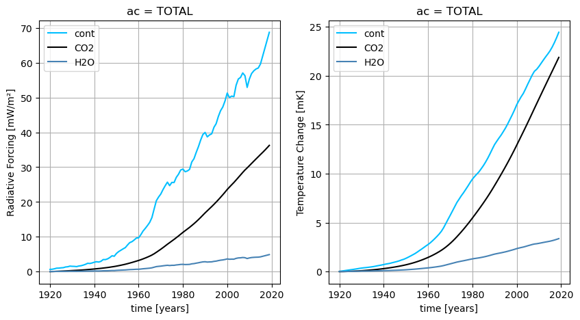
# Plot Radiative Forcing and Temperature Changes

ac = "TOTAL"
rf_cont = results_ds.RF_cont.sel(ac=ac) * 1000
rf_co2 = results_ds.RF_CO2.sel(ac=ac) * 1000
rf_h2o = results_ds.RF_H2O.sel(ac=ac) * 1000
dt_cont = results_ds.dT_cont.sel(ac=ac) * 1000
dt_co2 = results_ds.dT_CO2.sel(ac=ac) * 1000
dt_h2o = results_ds.dT_H2O.sel(ac=ac) * 1000

fig, ax = plt.subplots(ncols=2, figsize=(10,5))
ax[0].grid(True)
ax[1].grid(True)
rf_cont.plot(ax=ax[0], color="deepskyblue", label="cont")
rf_co2.plot(ax=ax[0], color="k", label="CO2")
rf_h2o.plot(ax=ax[0], color="steelblue", label="H2O")
dt_cont.plot(ax=ax[1], color="deepskyblue", label="cont")
dt_co2.plot(ax=ax[1], color="k", label="CO2")
dt_h2o.plot(ax=ax[1], color="steelblue", label="H2O")
ax[0].set_ylabel("Radiative Forcing [mW/m²]")
ax[1].set_ylabel("Temperature Change [mK]")
ax[0].legend()
ax[1].legend()
<matplotlib.legend.Legend at 0x7f453e8a1310>
Climate metrics
Absolute Global Temperature Potential (AGTP)
Absolute Global Warming Potential (AGWP)
Average Temperature Response (ATR)
metrics_ds = xr.load_dataset("source/demos/01_norm/results/historic_metrics.nc")
display(metrics_ds)
<xarray.Dataset> Size: 128B
Dimensions:        (species: 4)
Coordinates:
  * species        (species) <U5 80B 'CO2' 'cont' 'H2O' 'total'
Data variables:
    AGTP_100_1920  (species) float32 16B 0.02605 0.01742 0.00337 0.04685
    AGWP_100_1920  (species) float32 16B 1.272 1.738 0.1739 3.184
    ATR_100_1920   (species) float32 16B 0.006835 0.00583 0.001128 0.01379
Attributes: (1)- species: 4
- species(species)<U5'CO2' 'cont' 'H2O' 'total'
- long_name :
- species
array(['CO2', 'cont', 'H2O', 'total'], dtype='<U5')
- AGTP_100_1920(species)float320.02605 0.01742 0.00337 0.04685
- long_name :
- Absolute Global Temperature Change Potential
- units :
- K
- t_0 :
- 1920
- H :
- 100
array([0.02605442, 0.01742425, 0.00337026, 0.04684892], dtype=float32)
- AGWP_100_1920(species)float321.272 1.738 0.1739 3.184
- long_name :
- Absolute Global Warming Potential
- units :
- W m-2 year
- t_0 :
- 1920
- H :
- 100
array([1.272366 , 1.7375801 , 0.17394067, 3.1838868 ], dtype=float32)
- ATR_100_1920(species)float320.006835 0.00583 0.001128 0.01379
- long_name :
- Average Temperature Response
- units :
- K
- t_0 :
- 1920
- H :
- 100
array([0.00683476, 0.00583021, 0.0011277 , 0.01379268], dtype=float32)
- Title :
- historic climate metrics