Multiple emission inventories

In this example, no time evolution file is given, but multiple emission inventories are given as input. OpenAirClim will interpolate between discrete inventory years.

Imports

If the openairclim package cannot be imported, make sure that you have installed the package with pip or added the oac source folder to PYTHONPATH.

import xarray as xr
import matplotlib.pyplot as plt
import zenodo_get
import openairclim as oac

xr.set_options(display_expand_attrs=False)

<xarray.core.options.set_options at 0x7f484a09b0e0>

Input files

In order to be able to execute this example simulation, two types of input are required.

• Configuration file multi_inv.toml

• Emission inventories emi_inv_20XX.nc

Emission inventories

• Source: DLR research study DEPA 2050

• Inventory years: 2030, 2040, 2050

• Available for download in suitable OpenAirClim format

%%capture
# Download inventories from zenodo
zenodo_get.zenodo_get(["https://doi.org/10.5281/zenodo.11442322", "-g", "emi_inv_20[3-5]0.nc", "-o", "source/demos/input/"])

Simulation run

oac.run("source/demos/03_multi_inv/multi_inv.toml")

read_config ln. 254 in check_against_template INFO: Get default value for: responses CO2 rf method 

read_config ln. 254 in check_against_template INFO: Get default value for: responses cont method 

read_config ln. 520 in check_metrics_time ERROR: Metrics time settings with t_0 = 2020 and H = 21 are outside defined time range.

read_config ln. 532 in check_metrics_time WARNING: Last year in metrics time with t_0 = 2020 and H = 21 is earlier than last year in time range.

read_config ln. 185 in check_config ERROR: Configuration is not valid.

read_config ln. 376 in create_output_dir INFO: Create new output directory source/demos/03_multi_inv/results/

read_netcdf ln. 173 in open_inventories INFO: Emission inventories openend, attribute sections and time constraints checked successfully.

read_netcdf ln. 220 in split_inventory_by_aircraft WARNING: No ac coordinate found in emission inventory for year 2030. Reverting to 'DEFAULT' aircraft from config file.

read_netcdf ln. 220 in split_inventory_by_aircraft WARNING: No ac coordinate found in emission inventory for year 2040. Reverting to 'DEFAULT' aircraft from config file.

read_netcdf ln. 220 in split_inventory_by_aircraft WARNING: No ac coordinate found in emission inventory for year 2050. Reverting to 'DEFAULT' aircraft from config file.

main ln. 264 in run INFO: No subsequent species (PMO) defined in config.

main ln. 277 in run INFO: Execution time: 1.8726160526275635 sec

main ln. 280 in run WARNING: OpenAirClim is currently in development phase.
The computed output is not for scientific purposes until release of our publication.
Amongst others, the climate impact of longer species lifetimes in the stratosphere is not considered.

Results

Time series

• Emission sums

• Concentrations

• Radiative forcings

• Temperature changes

results_ds = xr.load_dataset("source/demos/03_multi_inv/results/multi_inv.nc")
display(results_ds)

<xarray.Dataset> Size: 4kB
Dimensions:        (ac: 2, time: 21)
Coordinates:
  * time           (time) int64 168B 2030 2031 2032 2033 ... 2047 2048 2049 2050
  * ac             (ac) <U7 56B 'DEFAULT' 'TOTAL'
Data variables:
    emis_CO2       (ac, time) float64 336B 1.075e+03 1.101e+03 ... 1.712e+03
    emis_distance  (ac, time) float64 336B 6.371e+10 6.478e+10 ... 8.757e+10
    emis_H2O       (ac, time) float64 336B 431.4 441.9 452.5 ... 671.8 686.8
    conc_CO2       (ac, time) float64 336B 0.1379 0.2718 0.4038 ... 2.823 2.984
    RF_CO2         (ac, time) float64 336B 0.001642 0.003213 ... 0.02954 0.03104
    RF_cont        (ac, time) float64 336B 0.04683 0.04708 ... 0.05769 0.05863
    RF_H2O         (ac, time) float64 336B 0.002381 0.002407 ... 0.003386
    dT_CO2         (ac, time) float64 336B 0.0001251 0.0003559 ... 0.01398
    dT_cont        (ac, time) float64 336B 0.002105 0.003987 ... 0.01958 0.02008
    dT_H2O         (ac, time) float64 336B 0.0002068 0.0003929 ... 0.002155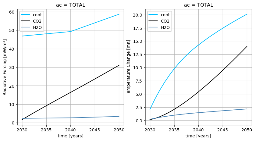
Attributes: (4)

xarray.Dataset

• Dimensions:
  • ac: 2
  • time: 21
• Coordinates: (2)
  • time
    (time)
    int64
    2030 2031 2032 ... 2048 2049 2050

    long_name :

    time

    units :

    years

    array([2030, 2031, 2032, 2033, 2034, 2035, 2036, 2037, 2038, 2039, 2040, 2041,
           2042, 2043, 2044, 2045, 2046, 2047, 2048, 2049, 2050])

  • ac
    (ac)
    <U7
    'DEFAULT' 'TOTAL'

    long_name :

    aircraft identifier

    array(['DEFAULT', 'TOTAL'], dtype='<U7')

• Data variables: (10)
  • emis_CO2
    (ac, time)
    float64
    1.075e+03 1.101e+03 ... 1.712e+03

    long_name :

    CO2 Emission

    units :

    Tg

    array([[1075.02554317, 1101.31766886, 1127.60979456, 1153.90192026,
            1180.19404595, 1206.48617165, 1232.77829734, 1259.07042304,
            1285.36254874, 1311.65467443, 1337.94680013, 1375.30528236,
            1412.66376458, 1450.02224681, 1487.38072904, 1524.73921126,
            1562.09769349, 1599.45617572, 1636.81465795, 1674.17314017,
            1711.5316224 ],
           [1075.02554317, 1101.31766886, 1127.60979456, 1153.90192026,
            1180.19404595, 1206.48617165, 1232.77829734, 1259.07042304,
            1285.36254874, 1311.65467443, 1337.94680013, 1375.30528236,
            1412.66376458, 1450.02224681, 1487.38072904, 1524.73921126,
            1562.09769349, 1599.45617572, 1636.81465795, 1674.17314017,
            1711.5316224 ]])

  • emis_distance
    (ac, time)
    float64
    6.371e+10 6.478e+10 ... 8.757e+10

    long_name :

    distance Emission

    units :

    km

    array([[6.37100278e+10, 6.47809647e+10, 6.58519015e+10, 6.69228384e+10,
            6.79937753e+10, 6.90647122e+10, 7.01356491e+10, 7.12065860e+10,
            7.22775228e+10, 7.33484597e+10, 7.44193966e+10, 7.57345198e+10,
            7.70496430e+10, 7.83647662e+10, 7.96798894e+10, 8.09950126e+10,
            8.23101358e+10, 8.36252590e+10, 8.49403822e+10, 8.62555054e+10,
            8.75706286e+10],
           [6.37100278e+10, 6.47809647e+10, 6.58519015e+10, 6.69228384e+10,
            6.79937753e+10, 6.90647122e+10, 7.01356491e+10, 7.12065860e+10,
            7.22775228e+10, 7.33484597e+10, 7.44193966e+10, 7.57345198e+10,
            7.70496430e+10, 7.83647662e+10, 7.96798894e+10, 8.09950126e+10,
            8.23101358e+10, 8.36252590e+10, 8.49403822e+10, 8.62555054e+10,
            8.75706286e+10]])

  • emis_H2O
    (ac, time)
    float64
    431.4 441.9 452.5 ... 671.8 686.8

    long_name :

    H2O Emission

    units :

    Tg

    array([[431.39065446, 441.94126889, 452.49188332, 463.04249774,
            473.59311217, 484.14372659, 494.69434102, 505.24495544,
            515.79556987, 526.34618429, 536.89679872, 551.88816527,
            566.87953183, 581.87089838, 596.86226493, 611.85363149,
            626.84499804, 641.8363646 , 656.82773115, 671.8190977 ,
            686.81046426],
           [431.39065446, 441.94126889, 452.49188332, 463.04249774,
            473.59311217, 484.14372659, 494.69434102, 505.24495544,
            515.79556987, 526.34618429, 536.89679872, 551.88816527,
            566.87953183, 581.87089838, 596.86226493, 611.85363149,
            626.84499804, 641.8363646 , 656.82773115, 671.8190977 ,
            686.81046426]])

  • conc_CO2
    (ac, time)
    float64
    0.1379 0.2718 ... 2.823 2.984

    long_name :

    CO2 Concentration

    units :

    ppmv

    array([[0.13794532, 0.27178481, 0.40379622, 0.53525637, 0.66688545,
            0.79909381, 0.93211907, 1.06610226, 1.20113011, 1.33725868,
            1.47452637, 1.61438128, 1.75676831, 1.90165372, 2.04901555,
            2.19883832, 2.35110999, 2.50582041, 2.66296035, 2.82252107,
            2.984494  ],
           [0.13794532, 0.27178481, 0.40379622, 0.53525637, 0.66688545,
            0.79909381, 0.93211907, 1.06610226, 1.20113011, 1.33725868,
            1.47452637, 1.61438128, 1.75676831, 1.90165372, 2.04901555,
            2.19883832, 2.35110999, 2.50582041, 2.66296035, 2.82252107,
            2.984494  ]])

  • RF_CO2
    (ac, time)
    float64
    0.001642 0.003213 ... 0.03104

    long_name :

    CO2 Radiative Forcing

    units :

    W/m²

    array([[0.00164236, 0.00321274, 0.00473941, 0.00623817, 0.00771795,
            0.00918384, 0.01063885, 0.01208478, 0.0135228 , 0.01495368,
            0.01637799, 0.01781048, 0.01925148, 0.02070045, 0.02215698,
            0.02362075, 0.02509149, 0.02656894, 0.02805286, 0.02954304,
            0.03103925],
           [0.00164236, 0.00321274, 0.00473941, 0.00623817, 0.00771795,
            0.00918384, 0.01063885, 0.01208478, 0.0135228 , 0.01495368,
            0.01637799, 0.01781048, 0.01925148, 0.02070045, 0.02215698,
            0.02362075, 0.02509149, 0.02656894, 0.02805286, 0.02954304,
            0.03103925]])

  • RF_cont
    (ac, time)
    float64
    0.04683 0.04708 ... 0.05769 0.05863

    long_name :

    cont Radiative Forcing

    units :

    W/m²

    array([[0.04683353, 0.04707616, 0.04731878, 0.04756141, 0.04780404,
            0.04804666, 0.04828929, 0.04853192, 0.04877454, 0.04901717,
            0.0492598 , 0.0501967 , 0.05113361, 0.05207052, 0.05300742,
            0.05394433, 0.05488123, 0.05581814, 0.05675504, 0.05769195,
            0.05862886],
           [0.04683353, 0.04707616, 0.04731878, 0.04756141, 0.04780404,
            0.04804666, 0.04828929, 0.04853192, 0.04877454, 0.04901717,
            0.0492598 , 0.0501967 , 0.05113361, 0.05207052, 0.05300742,
            0.05394433, 0.05488123, 0.05581814, 0.05675504, 0.05769195,
            0.05862886]])

  • RF_H2O
    (ac, time)
    float64
    0.002381 0.002407 ... 0.003386

    long_name :

    H2O Radiative Forcing

    units :

    W/m²

    array([[0.00238147, 0.00240682, 0.00243216, 0.00245751, 0.00248286,
            0.0025082 , 0.00253355, 0.0025589 , 0.00258424, 0.00260959,
            0.00263494, 0.00271008, 0.00278523, 0.00286038, 0.00293553,
            0.00301068, 0.00308582, 0.00316097, 0.00323612, 0.00331127,
            0.00338641],
           [0.00238147, 0.00240682, 0.00243216, 0.00245751, 0.00248286,
            0.0025082 , 0.00253355, 0.0025589 , 0.00258424, 0.00260959,
            0.00263494, 0.00271008, 0.00278523, 0.00286038, 0.00293553,
            0.00301068, 0.00308582, 0.00316097, 0.00323612, 0.00331127,
            0.00338641]])

  • dT_CO2
    (ac, time)
    float64
    0.0001251 0.0003559 ... 0.01398

    long_name :

    CO2 Temperature change

    units :

    K

    array([[0.00012509, 0.00035595, 0.00067754, 0.00107774, 0.00154645,
            0.00207508, 0.00265626, 0.00328356, 0.00395136, 0.00465474,
            0.00538936, 0.00615249, 0.00694176, 0.00775498, 0.00859022,
            0.00944571, 0.01031987, 0.01121128, 0.01211866, 0.01304087,
            0.01397685],
           [0.00012509, 0.00035595, 0.00067754, 0.00107774, 0.00154645,
            0.00207508, 0.00265626, 0.00328356, 0.00395136, 0.00465474,
            0.00538936, 0.00615249, 0.00694176, 0.00775498, 0.00859022,
            0.00944571, 0.01031987, 0.01121128, 0.01211866, 0.01304087,
            0.01397685]])

  • dT_cont
    (ac, time)
    float64
    0.002105 0.003987 ... 0.02008

    long_name :

    cont Temperature change

    units :

    K

    array([[0.00210462, 0.00398711, 0.00567241, 0.00718266, 0.00853752,
            0.00975443, 0.01084889, 0.01183464, 0.0127239 , 0.01352751,
            0.01425508, 0.01494637, 0.01560548, 0.01623611, 0.01684148,
            0.01742451, 0.01798774, 0.01853346, 0.01906368, 0.0195802 ,
            0.02008462],
           [0.00210462, 0.00398711, 0.00567241, 0.00718266, 0.00853752,
            0.00975443, 0.01084889, 0.01183464, 0.0127239 , 0.01352751,
            0.01425508, 0.01494637, 0.01560548, 0.01623611, 0.01684148,
            0.01742451, 0.01798774, 0.01853346, 0.01906368, 0.0195802 ,
            0.02008462]])

  • dT_H2O
    (ac, time)
    float64
    0.0002068 0.0003929 ... 0.002155

    long_name :

    H2O Temperature change

    units :

    K

    array([[0.00020678, 0.00039287, 0.00056059, 0.000712  , 0.00084894,
            0.00097304, 0.00108573, 0.0011883 , 0.00128189, 0.00136751,
            0.00144606, 0.00152265, 0.00159752, 0.00167087, 0.00174287,
            0.0018137 , 0.00188348, 0.00195234, 0.0020204 , 0.00208776,
            0.0021545 ],
           [0.00020678, 0.00039287, 0.00056059, 0.000712  , 0.00084894,
            0.00097304, 0.00108573, 0.0011883 , 0.00128189, 0.00136751,
            0.00144606, 0.00152265, 0.00159752, 0.00167087, 0.00174287,
            0.0018137 , 0.00188348, 0.00195234, 0.0020204 , 0.00208776,
            0.0021545 ]])

• Indexes: (2)
  • time
    PandasIndex

    PandasIndex(Index([2030, 2031, 2032, 2033, 2034, 2035, 2036, 2037, 2038, 2039, 2040, 2041,
           2042, 2043, 2044, 2045, 2046, 2047, 2048, 2049, 2050],
          dtype='int64', name='time'))

  • ac
    PandasIndex

    PandasIndex(Index(['DEFAULT', 'TOTAL'], dtype='object', name='ac'))

• Attributes: (4)

  title :

  multi_inv

  created :

  2025-09-25 09:24:23

  user :

  runner

  oac version :

  0.12.0

# Plot Radiative Forcing and Temperature Changes

ac = "TOTAL"
rf_cont = results_ds.RF_cont.sel(ac=ac) * 1000
rf_co2 = results_ds.RF_CO2.sel(ac=ac) * 1000
rf_h2o = results_ds.RF_H2O.sel(ac=ac) * 1000
dt_cont = results_ds.dT_cont.sel(ac=ac) * 1000
dt_co2 = results_ds.dT_CO2.sel(ac=ac) * 1000
dt_h2o = results_ds.dT_H2O.sel(ac=ac) * 1000

fig, ax = plt.subplots(ncols=2, figsize=(10,5))
ax[0].grid(True)
ax[1].grid(True)
rf_cont.plot(ax=ax[0], color="deepskyblue", label="cont")
rf_co2.plot(ax=ax[0], color="k", label="CO2")
rf_h2o.plot(ax=ax[0], color="steelblue", label="H2O")
dt_cont.plot(ax=ax[1], color="deepskyblue", label="cont")
dt_co2.plot(ax=ax[1], color="k", label="CO2")
dt_h2o.plot(ax=ax[1], color="steelblue", label="H2O")
ax[0].set_ylabel("Radiative Forcing [mW/m²]")
ax[1].set_ylabel("Temperature Change [mK]")
ax[0].legend()
ax[1].legend()

<matplotlib.legend.Legend at 0x7f4846b08a50>