Scaling

In this example, the time evolution of type scaling is demonstrated. In the scenario, the emissions increase linearly from the year 2019 to the year 2039. The emissions in 2039 are set to be twice as much as in 2019.

Imports

If the openairclim package cannot be imported, make sure that you have installed the package with pip or added the oac source folder to PYTHONPATH.

import xarray as xr
import matplotlib.pyplot as plt
import openairclim as oac

xr.set_options(display_expand_attrs=False)

<xarray.core.options.set_options at 0x7f7944cc17f0>

Input files

In order to be able to execute this example simulation, three types of input are required.

• Configuration file scaling.toml

• Emission inventories

  • ELK_aviation_2019_res5deg_flat.nc

  • ELK_aviation_2039_res5deg_flat.nc

• Time evolution file for scaling: time_scaling_linear_2019-2039.nc

Emission inventories

• Source: DLR Project EmissionsLandKarte (ELK)

• Resolution down-sampled to 5 deg resolution

• Converted into format suitable for OpenAirClim

• Inventory years

  • 2019 (original)

  • 2039 (same inventory as original, only year changed)

Time evolution

• Time evolution with scaling of emissions

• Time period: 2000 - 2050

• Linear ramp-up between years 2019 and 2039

evo = xr.load_dataset("source/demos/input/time_scaling_linear_2019-2039.nc")
display(evo)

fig, ax = plt.subplots()
evo.scaling.plot(ax=ax)
ax.grid(True)

<xarray.Dataset> Size: 408B
Dimensions:  (time: 51)
Coordinates:
  * time     (time) int32 204B 2000 2001 2002 2003 2004 ... 2047 2048 2049 2050
Data variables:
    scaling  (time) float32 204B 1.0 1.0 1.0 1.0 1.0 1.0 ... 2.0 2.0 2.0 2.0 2.0
Attributes: (5)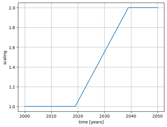

xarray.Dataset

• Dimensions:
  • time: 51
• Coordinates: (1)
  • time
    (time)
    int32
    2000 2001 2002 ... 2048 2049 2050

    units :

    years

    array([2000, 2001, 2002, 2003, 2004, 2005, 2006, 2007, 2008, 2009, 2010, 2011,
           2012, 2013, 2014, 2015, 2016, 2017, 2018, 2019, 2020, 2021, 2022, 2023,
           2024, 2025, 2026, 2027, 2028, 2029, 2030, 2031, 2032, 2033, 2034, 2035,
           2036, 2037, 2038, 2039, 2040, 2041, 2042, 2043, 2044, 2045, 2046, 2047,
           2048, 2049, 2050], dtype=int32)

• Data variables: (1)
  • scaling
    (time)
    float32
    1.0 1.0 1.0 1.0 ... 2.0 2.0 2.0 2.0

    species :

    all

    array([1.  , 1.  , 1.  , 1.  , 1.  , 1.  , 1.  , 1.  , 1.  , 1.  , 1.  ,
           1.  , 1.  , 1.  , 1.  , 1.  , 1.  , 1.  , 1.  , 1.  , 1.05, 1.1 ,
           1.15, 1.2 , 1.25, 1.3 , 1.35, 1.4 , 1.45, 1.5 , 1.55, 1.6 , 1.65,
           1.7 , 1.75, 1.8 , 1.85, 1.9 , 1.95, 2.  , 2.  , 2.  , 2.  , 2.  ,
           2.  , 2.  , 2.  , 2.  , 2.  , 2.  , 2.  ], dtype=float32)

• Attributes: (5)

  Title :

  Time scaling example

  Convention :

  CF-XXX

  Type :

  scaling

  Author :

  Stefan Völk

  Contact :

  stefan.voelk@dlr.de

Simulation run

oac.run("source/demos/02_scaling/scaling.toml")

Results

Time series

• Emission sums

• Concentrations

• Radiative forcings

• Temperature changes

results_ds = xr.load_dataset("source/demos/02_scaling/results/scaling.nc")
display(results_ds)

<xarray.Dataset> Size: 4kB
Dimensions:        (ac: 2, time: 21)
Coordinates:
  * ac             (ac) <U7 56B 'DEFAULT' 'TOTAL'
  * time           (time) int64 168B 2019 2020 2021 2022 ... 2036 2037 2038 2039
Data variables:
    emis_CO2       (ac, time) float64 336B 849.1 891.6 ... 1.656e+03 1.698e+03
    emis_distance  (ac, time) float64 336B 5.891e+10 6.185e+10 ... 1.178e+11
    emis_H2O       (ac, time) float64 336B 332.5 349.1 365.8 ... 648.4 665.0
    conc_CO2       (ac, time) float64 336B 0.109 0.2175 0.3272 ... 2.634 2.797
    RF_CO2         (ac, time) float64 336B 0.001705 0.003391 ... 0.03858 0.04083
    RF_cont        (ac, time) float64 336B 0.0664 0.06811 ... 0.09881 0.1005
    RF_H2O         (ac, time) float64 336B 0.004648 0.00488 ... 0.009296
    dT_CO2         (ac, time) float64 336B 0.0001299 0.0003738 ... 0.01773
    dT_cont        (ac, time) float64 336B 0.002984 0.005714 ... 0.03282 0.03376
    dT_H2O         (ac, time) float64 336B 0.0004036 0.0007826 ... 0.0057
Attributes: (4)

xarray.Dataset

• Dimensions:
  • ac: 2
  • time: 21
• Coordinates: (2)
  • ac
    (ac)
    <U7
    'DEFAULT' 'TOTAL'

    long_name :

    aircraft identifier

    array(['DEFAULT', 'TOTAL'], dtype='<U7')

  • time
    (time)
    int64
    2019 2020 2021 ... 2037 2038 2039

    long_name :

    time

    units :

    years

    array([2019, 2020, 2021, 2022, 2023, 2024, 2025, 2026, 2027, 2028, 2029, 2030,
           2031, 2032, 2033, 2034, 2035, 2036, 2037, 2038, 2039])

• Data variables: (10)
  • emis_CO2
    (ac, time)
    float64
    849.1 891.6 ... 1.656e+03 1.698e+03

    long_name :

    CO2 Emission

    units :

    Tg

    array([[ 849.14398041,  891.60113894,  934.0583987 ,  976.51555723,
            1018.97281698, 1061.42997551, 1103.88713404, 1146.3443938 ,
            1188.80155233, 1231.25881209, 1273.71597062, 1316.17312915,
            1358.6303889 , 1401.08754743, 1443.54480719, 1486.00196572,
            1528.45912425, 1570.91638401, 1613.37354254, 1655.83080229,
            1698.28796082],
           [ 849.14398041,  891.60113894,  934.0583987 ,  976.51555723,
            1018.97281698, 1061.42997551, 1103.88713404, 1146.3443938 ,
            1188.80155233, 1231.25881209, 1273.71597062, 1316.17312915,
            1358.6303889 , 1401.08754743, 1443.54480719, 1486.00196572,
            1528.45912425, 1570.91638401, 1613.37354254, 1655.83080229,
            1698.28796082]])

  • emis_distance
    (ac, time)
    float64
    5.891e+10 6.185e+10 ... 1.178e+11

    long_name :

    distance Emission

    units :

    km

    array([[5.89085988e+10, 6.18540260e+10, 6.47994601e+10, 6.77448872e+10,
            7.06903214e+10, 7.36357485e+10, 7.65811757e+10, 7.95266098e+10,
            8.24720369e+10, 8.54174711e+10, 8.83628982e+10, 9.13083254e+10,
            9.42537595e+10, 9.71991866e+10, 1.00144621e+11, 1.03090048e+11,
            1.06035475e+11, 1.08980909e+11, 1.11926336e+11, 1.14871771e+11,
            1.17817198e+11],
           [5.89085988e+10, 6.18540260e+10, 6.47994601e+10, 6.77448872e+10,
            7.06903214e+10, 7.36357485e+10, 7.65811757e+10, 7.95266098e+10,
            8.24720369e+10, 8.54174711e+10, 8.83628982e+10, 9.13083254e+10,
            9.42537595e+10, 9.71991866e+10, 1.00144621e+11, 1.03090048e+11,
            1.06035475e+11, 1.08980909e+11, 1.11926336e+11, 1.14871771e+11,
            1.17817198e+11]])

  • emis_H2O
    (ac, time)
    float64
    332.5 349.1 365.8 ... 648.4 665.0

    long_name :

    H2O Emission

    units :

    Tg

    array([[332.5074723 , 349.13283006, 365.75822746, 382.38358522,
            399.00898262, 415.63434038, 432.25969814, 448.88509553,
            465.51045329, 482.13585069, 498.76120845, 515.38656621,
            532.01196361, 548.63732137, 565.26271877, 581.88807653,
            598.51343429, 615.13883168, 631.76418944, 648.38958684,
            665.0149446 ],
           [332.5074723 , 349.13283006, 365.75822746, 382.38358522,
            399.00898262, 415.63434038, 432.25969814, 448.88509553,
            465.51045329, 482.13585069, 498.76120845, 515.38656621,
            532.01196361, 548.63732137, 565.26271877, 581.88807653,
            598.51343429, 615.13883168, 631.76418944, 648.38958684,
            665.0149446 ]])

  • conc_CO2
    (ac, time)
    float64
    0.109 0.2175 0.3272 ... 2.634 2.797

    long_name :

    CO2 Concentration

    units :

    ppmv

    array([[0.10896061, 0.21746125, 0.32715018, 0.43893466, 0.55331055,
            0.67054527, 0.79077945, 0.91408341, 1.04048842, 1.17000416,
            1.30262835, 1.43835214, 1.57716313, 1.71904692, 1.86398814,
            2.01197087, 2.162979  , 2.31699637, 2.47400679, 2.6339942 ,
            2.7969426 ],
           [0.10896061, 0.21746125, 0.32715018, 0.43893466, 0.55331055,
            0.67054527, 0.79077945, 0.91408341, 1.04048842, 1.17000416,
            1.30262835, 1.43835214, 1.57716313, 1.71904692, 1.86398814,
            2.01197087, 2.162979  , 2.31699637, 2.47400679, 2.6339942 ,
            2.7969426 ]])

  • RF_CO2
    (ac, time)
    float64
    0.001705 0.003391 ... 0.04083

    long_name :

    CO2 Radiative Forcing

    units :

    W/m²

    array([[0.0017052 , 0.00339127, 0.00508393, 0.00679725, 0.00853869,
            0.01031211, 0.01211936, 0.01395957, 0.01583411, 0.0177428 ,
            0.01968529, 0.02166114, 0.0236675 , 0.02570583, 0.02777561,
            0.02987632, 0.03200744, 0.03416845, 0.03635885, 0.03857815,
            0.04082586],
           [0.0017052 , 0.00339127, 0.00508393, 0.00679725, 0.00853869,
            0.01031211, 0.01211936, 0.01395957, 0.01583411, 0.0177428 ,
            0.01968529, 0.02166114, 0.0236675 , 0.02570583, 0.02777561,
            0.02987632, 0.03200744, 0.03416845, 0.03635885, 0.03857815,
            0.04082586]])

  • RF_cont
    (ac, time)
    float64
    0.0664 0.06811 ... 0.09881 0.1005

    long_name :

    cont Radiative Forcing

    units :

    W/m²

    array([[0.06640008, 0.06810578, 0.06981148, 0.07151717, 0.07322287,
            0.07492857, 0.07663426, 0.07833996, 0.08004566, 0.08175136,
            0.08345705, 0.08516275, 0.08686845, 0.08857415, 0.09027985,
            0.09198554, 0.09369124, 0.09539694, 0.09710263, 0.09880833,
            0.10051403],
           [0.06640008, 0.06810578, 0.06981148, 0.07151717, 0.07322287,
            0.07492857, 0.07663426, 0.07833996, 0.08004566, 0.08175136,
            0.08345705, 0.08516275, 0.08686845, 0.08857415, 0.09027985,
            0.09198554, 0.09369124, 0.09539694, 0.09710263, 0.09880833,
            0.10051403]])

  • RF_H2O
    (ac, time)
    float64
    0.004648 0.00488 ... 0.009296

    long_name :

    H2O Radiative Forcing

    units :

    W/m²

    array([[0.00464776, 0.00488015, 0.00511253, 0.00534492, 0.00557731,
            0.0058097 , 0.00604209, 0.00627447, 0.00650686, 0.00673925,
            0.00697164, 0.00720403, 0.00743641, 0.0076688 , 0.00790119,
            0.00813358, 0.00836597, 0.00859835, 0.00883074, 0.00906313,
            0.00929552],
           [0.00464776, 0.00488015, 0.00511253, 0.00534492, 0.00557731,
            0.0058097 , 0.00604209, 0.00627447, 0.00650686, 0.00673925,
            0.00697164, 0.00720403, 0.00743641, 0.0076688 , 0.00790119,
            0.00813358, 0.00836597, 0.00859835, 0.00883074, 0.00906313,
            0.00929552]])

  • dT_CO2
    (ac, time)
    float64
    0.0001299 0.0003738 ... 0.01773

    long_name :

    CO2 Temperature change

    units :

    K

    array([[0.00012988, 0.0003738 , 0.00071966, 0.00115778, 0.00168015,
            0.00227994, 0.00295125, 0.00368876, 0.00448787, 0.00534447,
            0.0062549 , 0.00721588, 0.00822429, 0.00927745, 0.01037298,
            0.01150869, 0.01268264, 0.01389304, 0.01513828, 0.01641689,
            0.01772754],
           [0.00012988, 0.0003738 , 0.00071966, 0.00115778, 0.00168015,
            0.00227994, 0.00295125, 0.00368876, 0.00448787, 0.00534447,
            0.0062549 , 0.00721588, 0.00822429, 0.00927745, 0.01037298,
            0.01150869, 0.01268264, 0.01389304, 0.01513828, 0.01641689,
            0.01772754]])

  • dT_cont
    (ac, time)
    float64
    0.002984 0.005714 ... 0.03376

    long_name :

    cont Temperature change

    units :

    K

    array([[0.00298391, 0.00571408, 0.00821909, 0.01052432, 0.01265229,
            0.01462301, 0.01645423, 0.0181617 , 0.01975941, 0.0212598 ,
            0.02267389, 0.02401145, 0.0252812 , 0.02649083, 0.0276472 ,
            0.02875638, 0.02982378, 0.03085419, 0.03185185, 0.03282054,
            0.03376362],
           [0.00298391, 0.00571408, 0.00821909, 0.01052432, 0.01265229,
            0.01462301, 0.01645423, 0.0181617 , 0.01975941, 0.0212598 ,
            0.02267389, 0.02401145, 0.0252812 , 0.02649083, 0.0276472 ,
            0.02875638, 0.02982378, 0.03085419, 0.03185185, 0.03282054,
            0.03376362]])

  • dT_H2O
    (ac, time)
    float64
    0.0004036 0.0007826 ... 0.0057

    long_name :

    H2O Temperature change

    units :

    K

    array([[0.00040356, 0.00078262, 0.00113996, 0.00147803, 0.00179903,
            0.00210491, 0.00239739, 0.00267801, 0.00294812, 0.00320893,
            0.00346151, 0.00370682, 0.00394571, 0.00417891, 0.00440709,
            0.00463086, 0.00485072, 0.00506716, 0.00528057, 0.00549132,
            0.00569976],
           [0.00040356, 0.00078262, 0.00113996, 0.00147803, 0.00179903,
            0.00210491, 0.00239739, 0.00267801, 0.00294812, 0.00320893,
            0.00346151, 0.00370682, 0.00394571, 0.00417891, 0.00440709,
            0.00463086, 0.00485072, 0.00506716, 0.00528057, 0.00549132,
            0.00569976]])

• Attributes: (4)

  title :

  scaling

  created :

  2025-11-19 10:54:25

  user :

  runner

  oac version :

  0.13.0

# Plot Radiative Forcing and Temperature Changes

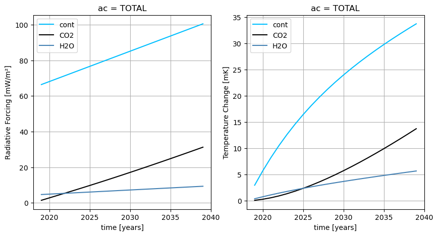
ac = "TOTAL"
rf_cont = results_ds.RF_cont.sel(ac=ac) * 1000
rf_co2 = results_ds.RF_CO2.sel(ac=ac) * 1000
rf_h2o = results_ds.RF_H2O.sel(ac=ac) * 1000
dt_cont = results_ds.dT_cont.sel(ac=ac) * 1000
dt_co2 = results_ds.dT_CO2.sel(ac=ac) * 1000
dt_h2o = results_ds.dT_H2O.sel(ac=ac) * 1000

fig, ax = plt.subplots(ncols=2, figsize=(10,5))
ax[0].grid(True)
ax[1].grid(True)
rf_cont.plot(ax=ax[0], color="deepskyblue", label="cont")
rf_co2.plot(ax=ax[0], color="k", label="CO2")
rf_h2o.plot(ax=ax[0], color="steelblue", label="H2O")
dt_cont.plot(ax=ax[1], color="deepskyblue", label="cont")
dt_co2.plot(ax=ax[1], color="k", label="CO2")
dt_h2o.plot(ax=ax[1], color="steelblue", label="H2O")
ax[0].set_ylabel("Radiative Forcing [mW/m²]")
ax[1].set_ylabel("Temperature Change [mK]")
ax[0].legend()
ax[1].legend()

<matplotlib.legend.Legend at 0x7f7943e0c050>